Gamedev Math · Thobias Høivik

Why game development?

Game development is one of the central gateways into programming.

I still remember being around twelve years old and my father trying to teach me some basic Java because I wanted to make Minecraft mods. I wrote Hello World, discovered that programming involved substantially more work than installing mods, and promptly abandoned the project.

Several years later I spent IT classes making games in JavaScript and thought for a while that game development might be what I wanted to do.

That is no longer the plan, but something arguably worse happened: I became more interested in how the things worked than in the finished games.

How does a flat monitor create the illusion of a three-dimensional world?

How does a game know two oddly-shaped objects have collided?

How can an enemy navigate around walls rather than sprint directly into one?

Those questions lead very quickly to linear algebra, computational geometry, graph algorithms, optimization, numerical methods, probability, and plenty more.

For maximal indoctrination, I highly recommend the

Sebastian Lague $\rightarrow$ Freya Holmér $\rightarrow$ 3Blue1Brown

pipeline.

Let us take a few things which appear almost effortless in a game and demystify them.

1. How does a computer draw a cube?

Behold, a cube!

Projection

Projection modeField of view: 55°Camera distance: 4.4

Interaction

Auto rotate

Drag the cube to rotate it. The scene is small because large scenes get really slow when rendered in the manner used here. I have a really old project on GitHub which illustrates this.

Spin it around. Try the different projection modes.

This does not seem all that profound or interesting, it is just a cube.

Except that your screen has a serious limitation. That being that

it is flat.

The object appears to live in three dimensions, while the browser eventually has to decide which two-dimensional pixels to draw.

So somewhere inside the demo we need a procedure which does roughly the following.

\text{3D world} \longrightarrow \text{2D image}.

A cube is really just some points

For our tiny renderer, it is enough to store the cube’s eight corners and remember which corners belong to which faces.

A position in three-dimensional space can be described using three numbers:

(x,y,z).

For the cube in the demo, each coordinate starts as either $-1$ or $1$ .

So the eight corners are simply all the possibilities

(\pm1,\pm1,\pm1).

For example,

(1,-1,1)

just describes one particular point in space.

What happens every frame?

Roughly speaking, the procedure looks something like this:

start with the cube’s vertices,
move them according to the cube’s rotation,
describe them relative to the camera,
project the three-dimensional points onto a two-dimensional screen,
connect the projected points into faces,
draw those faces.

The rotating solid object you see is therefore really a collection of numbers being transformed over and over again.

But this is just linear algebra!

What does “rotate the cube” mean to a computer?

Suppose I rotate the cube a little to the right.

Every corner moves. The corners cannot move independently.

They have to move together in exactly the coordinated way which keeps the object rigid.

So we want a rule to transform the positions of points, preserving their distance and relative positions.

Matrices give us an nice compact way to represent such transformations.

You do not need to understand a rotation matrix to understand the renderer, in fact one can perfor $3$ elementary transformations to each position vector one after the other to achieve the result, but matrices can compactly store all $3$ transformations you need.

What does the rotation matrix actually do?

A rotation by an angle $\theta$ around the $y$ -axis can be represented by

R_y(\theta) = \begin{pmatrix} \cos\theta & 0 & \sin\theta \\ 0 & 1 & 0 \\ -\sin\theta & 0 & \cos\theta \end{pmatrix}.

If a vertex has coordinates

v= \begin{pmatrix} x\\ y\\ z \end{pmatrix},

then its rotated position is

R_y(\theta)v.

Multiplying this out gives

x' = x\cos\theta+z\sin\theta,

y'=y,

and

z' = -x\sin\theta+z\cos\theta.

Notice that the $y$ -coordinate does not change.

That is exactly what we should expect: rotating around the $y$ -axis moves points around that axis rather than along it.

If transformations like this seem interesting, the linear transformations lab goes into why matrices behave this way!

Perspective

Now we run into another problem.

Take two objects of exactly the same physical size.

Put one beside you and the other far away.

The distant object looks smaller.

A perspective renderer has to manufacture the same effect.

The idea of the trick is quite simple!

For a point

(x,y,z),

a simple perspective projection looks roughly like

x_{\mathrm{screen}} \sim \frac{x}{z}, \qquad y_{\mathrm{screen}} \sim \frac{y}{z}.

Look only at the denominator.

When the depth $z$ becomes larger, the projected coordinates become smaller.

So points farther away are pulled toward the centre of the image.

So we simply divide by depth!

Make the projection a little more precise

For an idealized pinhole camera with focal length $f$ , one common convention gives

x_{\mathrm{screen}} = f\frac{x}{z}, \qquad y_{\mathrm{screen}} = f\frac{y}{z}.

Real graphics pipelines usually package perspective projection into a projection matrix and use homogeneous coordinates.

A typical pipeline moves through several coordinate systems:

\text{model space} \to \text{world space} \to \text{camera space} \to \text{clip space} \to \text{screen space}.

Model space describes the object relative to itself.

World space places it into the scene.

Camera space describes everything relative to the camera.

Projection produces clip coordinates, followed by perspective division and viewport mapping to obtain screen coordinates.

Orthographic projection removes the shrinking-with-distance effect.

That makes it useful for technical drawings, editors, some strategy games, isometric-looking scenes, and other places where perspective is undesirable. Remember those cool full-world screen shots you could take in Minecraft back in the day? Those used orthographic projection!

Triangles, triangles, triangles

Our cube appears to have six square faces.

But the renderer can split each square into two triangles.

We do this because triangles are convenient, being the simplest convex polygons.

Furthermore, three non-collinear points determine a unique plane, while a polygon with four or more vertices can be troublesome because its vertices do not even have to lie in the same plane.

So real-time graphics overwhelmingly represents surfaces using triangle meshes.

Our cube needs only

6 \times 2 = 12

triangles.

A detailed character may use tens or hundreds of thousands.

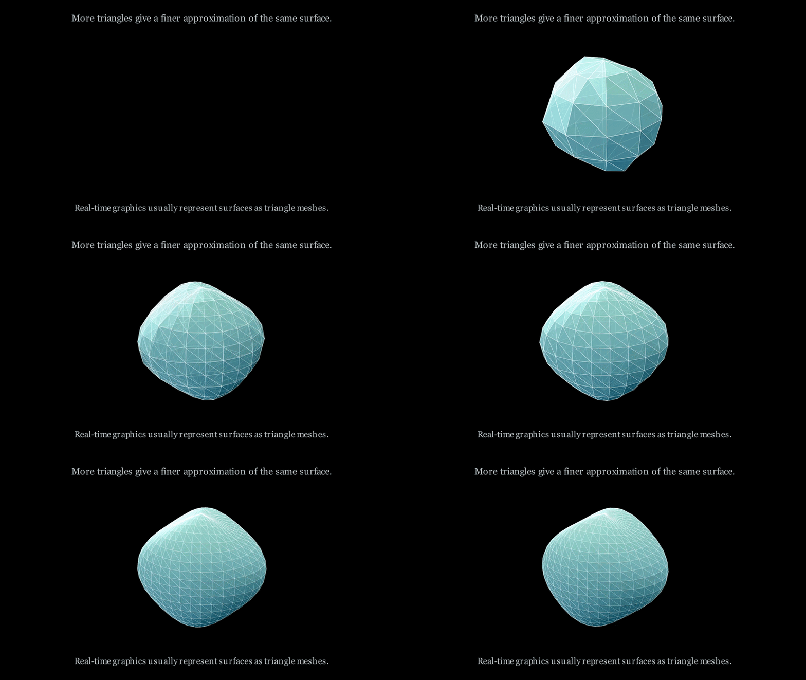
A triangulated mesh increasing in detail — Triangle count increasing on a simple mesh.

Once a world is decomposed into triangles, the renderer can simply determine which pixels the triangle covers and what they should look like, over and over.

What does a real renderer do after this?

A modern rasterization pipeline typically performs substantially more work than the little demo on this page.

Triangles may be clipped against the camera’s viewing region, transformed into screen space, rasterized into fragments, shaded, depth-tested, blended, and finally written to the framebuffer.

The cube demo is deliberately primitive.

It uses Canvas 2D, sorts faces by depth, and draws them back-to-front. This is a version of the painter’s algorithm.

That works for a cube, but it is not robust for arbitrary three-dimensional scenes.

A serious renderer normally uses a depth buffer rather than relying only on drawing order.

The important idea to keep is

\text{points in 3D} \to \text{move the points} \to \text{project them} \to \text{fill triangles}.

Graphics rabbit holes

My own first serious attempt at understanding rendering from scratch came from Software Rendering from Scratch.

Some other resources I like:

2. Collision detection!

Move these two shapes around:

Collision

Orientation

Rectangle A: 18°Rectangle B: -24°

SAT axis

Overlap: 0.27

Axis from rectangle B

Experiment

Show candidate axes

Drag either rectangle. Auto mode displays a separating axis when one exists; during a collision it shows the axis of least penetration.

You can look at them and immediately say whether they overlap.

Computers however, are stupid, so we need an explicit test.

For arbitrary shapes this can become quite difficult.

For convex polygons, however, some mathematician (the great Hermann Minkowski) has done the work for us!

Look at the shadows

Imagine choosing some direction and projecting both polygons onto a line.

You can think of this as shining light (placed infinitely far away!) on them and looking only at their shadows.

Now suppose the two shadows do not overlap.

Then the original polygons cannot overlap either.

There is a direction from which we can literally see a gap between them.

So instead of directly solving the two-dimensional problem of asking whether the polygons intersect, we try to solve a collection of much easier one-dimensional problems “are these intervals intersecting”.

If we find even one direction where the projected intervals are separate, the polygons are separate.

Such a direction is called a separating axis.

That is the central idea behind the Separating Axis Theorem, or SAT (not to be confused with boolean satifiability!).

Try moving the shapes back in the demo until they separate.

The demo highlights an axis for which there is a gap.

illustration showing collision detection via shadows — See how we can find a direction where the shadows don't overlap!

Why don’t we need to check every possible direction?

There are infinitely many directions in the plane, which is unpractical.

Fortunately, for convex polygons we only need a small collection of candidates.

It is enough to test directions perpendicular to the edges of the polygons.

So a polygon with a small number of edges gives us only a small number of shadow tests.

Make the shadow idea precise

Choose an axis represented by a unit vector $n$ .

A point $x$ is projected onto this axis using the dot product

x \longmapsto x\cdot n.

A convex polygon $A$ therefore projects to the interval

I_A(n) = \left[ \min_{a\in A} a\cdot n, \max_{a\in A} a\cdot n \right].

Similarly,

I_B(n) = \left[ \min_{b\in B} b\cdot n, \max_{b\in B} b\cdot n \right].

If for some candidate axis $n$ ,

I_A(n)\cap I_B(n)=\varnothing,

then $A$ and $B$ do not intersect.

For convex polygons in two dimensions, if the polygons are disjoint, such a separating axis exists among the normals to their edges.

Detecting a collision is only half the job

Suppose the two shapes overlap.

Great. We have detected the problem.

Unfortunately, the player is now inside the wall.

A game usually needs to figure out how to separate them again.

The shadow calculation gives us useful information for this too.

When the polygons overlap, their projected intervals overlap along every candidate axis.

But not necessarily by the same amount.

Along one direction the shadows might overlap a lot.

Along another they might overlap only slightly.

The direction requiring the smallest useful push gives us a natural way to separate the shapes.

Press Resolve collision in the demo and watch which way the algorithm moves them.

Penetration depth and the minimum translation vector

For each candidate axis, we compute the overlap between the projected intervals.

With the usual SAT bookkeeping, the smallest penetration depth determines a candidate direction in which one polygon can be translated out of the other with minimal movement.

That direction together with the required distance is commonly called a minimum translation vector.

A real rigid-body physics engine must then handle substantially more:

velocity,
mass,
impulses,
friction,
angular velocity,
multiple simultaneous contacts,
resting contacts,
numerical stability.

So collision detection is only the beginning of collision response.

Still, it is remarkable how much of the basic two-dimensional collision problem reduces to asking whether little intervals on a line overlap!

3. How does an enemy find you?

Suppose an enemy is standing on the other side of a level.

It wants to reach the player.

There are walls in the way.

To us, the task looks like movement through a map.

Again, the computer needs something more explicit.

So we throw away most of the visual information.

Every location the enemy is allowed to occupy becomes a vertex.

Whenever the enemy can move directly between two locations, connect those vertices by an edge.

The map has now become a network.

Also, we have nicely restated the question as asking what the shortest path from one point to another is.

Luckily for us, that problem has already been extensively stuied by theoretical computer scientists!

Try the four algorithms below after placing some walls and “expensive” cells. Note: This ran horribly on my phone so it might be a bit laggy on some systems, sorry!

Ready to search

Algorithm

Purple cells are currently in the frontier; cyan cells have already been expanded.

Edit grid

Animation speed: 70

Drag S and G to move the endpoints. Drag elsewhere to paint the selected terrain.

Watch where they explore.

There is one observation which makes all four considerably easier to understand, that being that they only really disagree on where they should explore next.

As you might see, this fundamental disagreement leads to quiet different behavior. If you look at the top right you can see how “expensive” each algorithm is when it comes to distance. Note also that some of the algorithms are faster than others. These are tradeoffs which will be elucidated below.

Breadth-first search

Suppose every move costs exactly the same amount.

Then the problem is simply to minimize the number of moves.

Breadth-first search, or BFS, expands outward from the starting point like a wave.

It first explores everything one step away.

Then everything two steps away.

Then three, and so on.

Because of this, the first time BFS reaches the goal, it has found a route using the minimum possible number of edges.

The data structure underneath this behaviour is the humble queue.

Newly discovered locations go to the back.

The oldest waiting location is explored next.

What is BFS doing formally?

For an unweighted graph

G=(V,E),

BFS computes shortest-path distances from a source $s$ measured by number of edges.

Using an adjacency-list representation, its running time is

O(|V|+|E|).

Each vertex is discovered at most once, and every edge is inspected only a constant number of times.

BFS is not a bad algorithm.

For unweighted shortest paths, it is often exactly the algorithm you want.

Its limitation appears when different movements have different costs.

What if some terrain is expensive?

Imagine a map where moving through ordinary ground costs $1$ .

Moving through mud costs $5$ .

Now the route using the fewest steps is not necessarily the cheapest route.

A short path through a swamp may cost more than a slightly longer path around it.

Try placing a thick strip of expensive cells between the start and goal in the demo if you haven’t already.

BFS is completely blind to this and only counts moves.

We now want an algorithm that cares about cost.

Dijkstra: explore the cheapest place reached so far

Dijkstra’s algorithm
(yes the one in your first discrete math course) changes the rule for deciding what to explore next.

Instead of asking which tike was discovered first, it asks which of the discovered tiles form the cheapest route thus far.

To efficiently keep track of “whichever thing currently has the smallest cost,” we typically use a priority queue.

For graphs with non-negative edge weights, Dijkstra’s algorithm finds shortest paths.

Dijkstra in notation

Let $d(v)$ denote the smallest currently-known cost of reaching $v$ from the source.

At each step, Dijkstra extracts an unsettled vertex minimizing

d(v).

Equivalently, we repeatedly choose something of the form

v = \operatorname*{arg\,min}_{u} d(u).

Edges are then relaxed: if travelling through $v$ gives a cheaper route to a neighbour $w$ , we update the estimate for $w$ .

With non-negative edge weights, once a vertex is removed from the priority queue with its minimum key in the standard algorithm, its shortest-path distance is settled.

Dijkstra is good at using information about the journey so far.

However, it ignores something which is obvious to us who have eyeballs.

It knows how much the journey has cost.

It does not inherently care which direction the goal lies.

Greedy search, i.e. the stubborn approach

Suppose the goal is clearly east of the enemy.

Spending lots of time exploring far to the west feels wasteful.

So what if we estimate how far every location appears to be from the goal?

That estimate is called a heuristic.

Greedy best-first search takes this idea to the extreme:

explore whichever location currently looks closest to the goal.

This can make it race toward the target.

This stupidity often leads to ridiculously bad decisions.

A wall may force us to travel away from the goal before we can eventually reach it.

Greedy search does not care how expensive the journey has already been.

It only cares about where the goal appears to be.

That is why it can be fast without necessarily finding an optimal path.

In essence, dumb, but fast!

A*, the best of both worlds

Dijkstra asks cares about cost, while Greedy cares about raw distance to the goal.

A* combines both ideas.

For every candidate location, A* combines

the cost already paid to reach it,
an estimate of the cost still remaining.

A location is attractive when the total cost is small.

This lets A* focus much more strongly toward the goal than Dijkstra while, with an appropriate heuristic, still preserving optimality.

The A* formula

A* assigns each vertex a score

f(v) = g(v)+h(v),

where

g(v)

is the best known cost from the start to $v$ , and

h(v)

is an estimate of the remaining cost from $v$ to the goal.

On a four-directional grid, a common choice is the Manhattan-distance (think about why it is called the Manhattan-distance! It is also often referred to as the Taxi-cab metric!) heuristic

h(v) = |x_v-x_t| + |y_v-y_t|.

If every move costs at least $1$ , this does not overestimate the true remaining cost.

More generally, appropriate admissibility and consistency conditions on the heuristic allow standard versions of A* to retain shortest-path optimality.

Greedy best-first search may be viewed as prioritizing only

h(v),

while Dijkstra may be viewed as using only

g(v).

A* combines the two.

So the four behaviours in the demo can be summarized surprisingly compactly:

\begin{array}{rcl} \text{BFS} &:& \text{explore by number of steps} \\[4pt] \text{Dijkstra} &:& \text{explore by cost so far} \\[4pt] \text{Greedy} &:& \text{explore by estimated distance remaining} \\[4pt] A^\ast &:& \text{combine cost so far with estimated cost remaining} \end{array}

More things I want to add

There are many other game-development techniques which have the same flavour.

Procedural noise starts from smooth interpolation and layered pseudo-randomness and somehow turns into terrain, clouds, textures and worlds.

Wave function collapse looks vaguely quantum-inspired from the name, but algorithmically it is much closer to constraint satisfaction: each local choice removes possibilities from neighbouring cells.

Marching squares and marching cubes turn sampled scalar fields into contours and surfaces. The technique began in scientific and medical visualization and is now familiar from games and procedural geometry.

Boids produce remarkably convincing flocking from a few local rules such as separation, alignment and cohesion.

Cellular automata generate complex global behaviour from tiny local update rules, from Conway’s Game of Life all the way toward wonderfully chaotic systems such as Noita’s pixel physics.